Show code
library(readxl)
library(dplyr)
library(tidyr)
library(knitr)
library(ggplot2)We begin by loading the packages used throughout this replication.
library(readxl)
library(dplyr)
library(tidyr)
library(knitr)
library(ggplot2)This file attempts to replicate the five mediation models from Boos et al. (2025) using the PediBIRN subset available in ../Data/Data.xlsx.
Because the full analytic codebook and the full 973-record paper dataset were not shared, this replication necessarily involves a few explicit assumptions:
severe_retinal_injury = 1 if retinoschisis or severe retinal hemorrhage is present.isolated_inertial_injury as the primary exposure, with diffuse_HIE and extra_axial_blood as mediators, based on the paper abstract and the intern reconstruction document.The goal is therefore not an identical reproduction of the published coefficients, but a transparent subset-based replication of the same basic causal model.
We now load the control and intervention sheets from the PediBIRN subset and combine them into a single patient-level dataset.
data_path <- "../Data/Data.xlsx"

dat_control <- read_excel(data_path, sheet = "Eligible Control Patients") |>
  mutate(data_source = "control")

dat_intervention <- read_excel(data_path, sheet = "Eligible Intervention Patients") |>
  mutate(data_source = "intervention")

dat_raw <- bind_rows(dat_control, dat_intervention)

nrow(dat_raw)
[1] 432This subset contains fewer records than the published paper dataset, so the coefficients should be treated as approximate rather than expected to match exactly.
We now reconstruct the mediation-model variables using the mappings described in Boos2025.pdf and the intern reconstruction document.
col_prefix <- function(prefix) {
  match_idx <- which(startsWith(names(dat_raw), prefix))[1]
  if (is.na(match_idx)) {
    stop(paste("No column found with prefix:", prefix))
  }
  names(dat_raw)[match_idx]
}

col_contains <- function(text) {
  match_idx <- grep(text, names(dat_raw), ignore.case = TRUE)[1]
  if (is.na(match_idx)) {
    stop(paste("No column found containing:", text))
  }
  names(dat_raw)[match_idx]
}

feature_map <- c(
  age_months = col_prefix("Q2.3.1."),
  respiratory_compromise = col_prefix("Q4.2.1."),
  circulatory_compromise = col_prefix("Q4.2.2."),
  seizure = col_prefix("Q4.2.3."),
  altered_consciousness = col_prefix("Q4.2.4."),
  loc_resolved_before_admission = col_prefix("Q4.2.5."),
  loc_gt24h = col_prefix("Q4.2.6."),
  loc_posturing = col_prefix("Q4.2.7."),
  craniofacial_injury = col_prefix("Q4.3.1."),
  skull_fracture = col_prefix("Q4.4.1."),
  epidural_hemorrhage = col_prefix("Q4.4.3."),
  subdural_hemorrhage = col_prefix("Q4.4.4."),
  sdh_bilateral = col_prefix("Q4.4.5.2."),
  sdh_interhemispheric = col_contains("interhemispheric space"),
  subarachnoid_hemorrhage = col_prefix("Q4.4.7."),
  hie_any = col_prefix("Q4.4.12."),
  hie_depth = col_prefix("Q4.4.13."),
  hie_distribution = col_prefix("Q4.4.14."),
  ophthalmology_eval = col_prefix("Q5.3.1.10."),
  retinoschisis = col_prefix("Q5.3.2.8."),
  severe_rh = col_prefix("Q5.3.2.9.")
)

mediation_data <- dat_raw |>
  transmute(
    age_months = as.numeric(.data[[feature_map["age_months"]]]),
    respiratory_compromise = as.integer(.data[[feature_map["respiratory_compromise"]]]),
    circulatory_compromise = as.integer(.data[[feature_map["circulatory_compromise"]]]),
    seizure = as.integer(.data[[feature_map["seizure"]]]),
    altered_consciousness = as.integer(.data[[feature_map["altered_consciousness"]]]),
    loc_resolved_before_admission = as.integer(.data[[feature_map["loc_resolved_before_admission"]]]),
    loc_gt24h = as.integer(.data[[feature_map["loc_gt24h"]]]),
    loc_posturing = as.integer(.data[[feature_map["loc_posturing"]]]),
    craniofacial_injury = as.integer(.data[[feature_map["craniofacial_injury"]]]),
    skull_fracture = as.integer(.data[[feature_map["skull_fracture"]]]),
    epidural_hemorrhage = as.integer(.data[[feature_map["epidural_hemorrhage"]]]),
    subdural_hemorrhage = as.integer(.data[[feature_map["subdural_hemorrhage"]]]),
    sdh_bilateral = as.integer(.data[[feature_map["sdh_bilateral"]]]),
    sdh_interhemispheric = as.integer(.data[[feature_map["sdh_interhemispheric"]]]),
    subarachnoid_hemorrhage = as.integer(.data[[feature_map["subarachnoid_hemorrhage"]]]),
    hie_any = as.integer(.data[[feature_map["hie_any"]]]),
    hie_depth = as.integer(.data[[feature_map["hie_depth"]]]),
    hie_distribution = as.integer(.data[[feature_map["hie_distribution"]]]),
    ophthalmology_eval = as.integer(.data[[feature_map["ophthalmology_eval"]]]),
    retinoschisis = as.integer(.data[[feature_map["retinoschisis"]]]),
    severe_rh = as.integer(.data[[feature_map["severe_rh"]]])
  ) |>
  mutate(
    severe_retinal_injury = if_else(
      ophthalmology_eval == 1L,
      if_else(retinoschisis == 1L | severe_rh == 1L, 1L, 0L),
      NA_integer_
    ),
    clinical_hypoxia_ischemia = if_else(
      respiratory_compromise == 1L | circulatory_compromise == 1L,
      1L, 0L,
      missing = NA_integer_
    ),
    duration_altered_consciousness = case_when(
      is.na(altered_consciousness) ~ NA_real_,
      altered_consciousness == 0L ~ 0,
      loc_resolved_before_admission == 1L ~ 1,
      altered_consciousness == 1L & loc_gt24h == 0L ~ 2,
      altered_consciousness == 1L & loc_gt24h == 1L & loc_posturing == 0L ~ 3,
      altered_consciousness == 1L & loc_gt24h == 1L & loc_posturing == 1L ~ 4,
      TRUE ~ NA_real_
    ),
    extra_axial_blood = if_else(
      subdural_hemorrhage == 1L | subarachnoid_hemorrhage == 1L,
      1L, 0L,
      missing = NA_integer_
    ),
    diffuse_HIE = if_else(
      hie_any == 1L & (hie_depth == 2L | hie_distribution == 2L),
      1L, 0L,
      missing = NA_integer_
    ),
    inertial_subdural = if_else(
      subdural_hemorrhage == 1L & (sdh_bilateral == 1L | sdh_interhemispheric == 1L),
      1L, 0L,
      missing = NA_integer_
    ),
    inertial_injury = if_else(
      altered_consciousness == 1L | inertial_subdural == 1L,
      1L, 0L,
      missing = NA_integer_
    ),
    contact_injury = if_else(
      craniofacial_injury == 1L | skull_fracture == 1L | epidural_hemorrhage == 1L,
      1L, 0L,
      missing = NA_integer_
    ),
    isolated_inertial_injury = if_else(
      inertial_injury == 1L & contact_injury == 0L,
      1L, 0L,
      missing = NA_integer_
    )
  )

analysis_vars <- c(
  "severe_retinal_injury",
  "isolated_inertial_injury",
  "inertial_injury",
  "clinical_hypoxia_ischemia",
  "diffuse_HIE",
  "duration_altered_consciousness",
  "extra_axial_blood",
  "seizure"
)

oph_subset <- mediation_data |>
  filter(ophthalmology_eval == 1L)

summary_tbl <- tibble(
  variable = analysis_vars,
  n_non_missing = sapply(oph_subset[analysis_vars], function(x) sum(!is.na(x))),
  mean = sapply(oph_subset[analysis_vars], function(x) mean(x, na.rm = TRUE))
)

kable(summary_tbl, digits = 3, caption = "Table 1. Reconstructed mediation-model variables in the ophthalmology subset")| variable | n_non_missing | mean |
|---|---|---|
| severe_retinal_injury | 313 | 0.428 |
| isolated_inertial_injury | 313 | 0.342 |
| inertial_injury | 313 | 0.815 |
| clinical_hypoxia_ischemia | 312 | 0.522 |
| diffuse_HIE | 313 | 0.355 |
| duration_altered_consciousness | 312 | 1.587 |
| extra_axial_blood | 313 | 0.907 |
| seizure | 312 | 0.407 |
This table checks that the reconstructed variables behave plausibly in the ophthalmology subset before any mediation modeling is attempted.
We now fit Model A, using isolated inertial injury as the exposure, diffuse HIE and extra-axial blood as mediators, and severe retinal injury as the outcome.
Statistically, this is implemented here as three logistic regression models. Let (X_i) denote isolated inertial injury for child (i), let (M_{1i}) denote diffuse HIE, let (M_{2i}) denote extra-axial blood, and let (Y_i) denote severe retinal injury. The fitted models are:
\[ \text{logit}\{\Pr(M_{1i} = 1)\} = \alpha_0 + \alpha_1 X_i + \varepsilon_{1i} \]
\[ \text{logit}\{\Pr(M_{2i} = 1)\} = \gamma_0 + \gamma_1 X_i + \varepsilon_{2i} \]
\[ \text{logit}\{\Pr(Y_i = 1)\} = \beta_0 + \beta_1 X_i + \beta_2 M_{1i} + \beta_3 M_{2i} + \varepsilon_{3i} \]
Under this approximation, the direct effect is represented by (_1), while the two indirect effects are summarized by the coefficient products (_1 _2) and (_1 _3).
We now show the same model as a directed acyclic graph.
model_a_data <- oph_subset |>
  select(all_of(c("severe_retinal_injury", "isolated_inertial_injury", "diffuse_HIE", "extra_axial_blood"))) |>
  na.omit()

mediator_model_diffuse_hie <- glm(
  diffuse_HIE ~ isolated_inertial_injury,
  data = model_a_data,
  family = binomial()
)

mediator_model_extra_axial <- glm(
  extra_axial_blood ~ isolated_inertial_injury,
  data = model_a_data,
  family = binomial()
)

outcome_model <- glm(
  severe_retinal_injury ~ isolated_inertial_injury + diffuse_HIE + extra_axial_blood,
  data = model_a_data,
  family = binomial()
)
This approximation uses logistic regression for both mediators and the outcome, then summarizes indirect effects as products of the relevant log-odds coefficients.
We now extend the same approximation to four additional inferred models so the document covers the full A-E set discussed in the paper. Because the exact figure definitions were not recoverable from the shared materials, these model specifications should be read as transparent approximations rather than exact reproductions.
model_specs <- tibble(
  model = c("A", "B", "C", "D", "E"),
  exposure = c(
    "isolated_inertial_injury",
    "inertial_injury",
    "diffuse_HIE",
    "diffuse_HIE",
    "clinical_hypoxia_ischemia"
  ),
  mediators = list(
    c("diffuse_HIE", "extra_axial_blood"),
    c("extra_axial_blood", "clinical_hypoxia_ischemia", "diffuse_HIE", "seizure"),
    c("duration_altered_consciousness", "extra_axial_blood", "clinical_hypoxia_ischemia", "seizure"),
    c("duration_altered_consciousness", "clinical_hypoxia_ischemia", "extra_axial_blood", "seizure"),
    c("duration_altered_consciousness", "diffuse_HIE", "seizure", "extra_axial_blood")
  ),
  description = c(
    "Isolated inertial injury with diffuse HIE and extra-axial blood as mediators.",
    "Inertial injury with or without contact injury, mediated through extra-axial blood, clinical hypoxia or ischemia, diffuse HIE, and seizure.",
    "Diffuse HIE mediated through duration of altered consciousness, extra-axial blood, clinical hypoxia or ischemia, and seizure.",
    "Diffuse HIE versus no HIE or focal HIE, mediated through duration of altered consciousness, clinical hypoxia or ischemia, extra-axial blood, and seizure.",
    "Clinical hypoxia or ischemia mediated through duration of altered consciousness, diffuse HIE, seizure, and extra-axial blood."
  )
)

model_specs_display <- model_specs |>
  mutate(mediators = vapply(mediators, paste, collapse = ", ", character(1)))

kable(model_specs_display, caption = "Table 2. Published Figure A-E specifications used in this replication")| model | exposure | mediators | description |
|---|---|---|---|
| A | isolated_inertial_injury | diffuse_HIE, extra_axial_blood | Isolated inertial injury with diffuse HIE and extra-axial blood as mediators. |
| B | inertial_injury | extra_axial_blood, clinical_hypoxia_ischemia, diffuse_HIE, seizure | Inertial injury with or without contact injury, mediated through extra-axial blood, clinical hypoxia or ischemia, diffuse HIE, and seizure. |
| C | diffuse_HIE | duration_altered_consciousness, extra_axial_blood, clinical_hypoxia_ischemia, seizure | Diffuse HIE mediated through duration of altered consciousness, extra-axial blood, clinical hypoxia or ischemia, and seizure. |
| D | diffuse_HIE | duration_altered_consciousness, clinical_hypoxia_ischemia, extra_axial_blood, seizure | Diffuse HIE versus no HIE or focal HIE, mediated through duration of altered consciousness, clinical hypoxia or ischemia, extra-axial blood, and seizure. |
| E | clinical_hypoxia_ischemia | duration_altered_consciousness, diffuse_HIE, seizure, extra_axial_blood | Clinical hypoxia or ischemia mediated through duration of altered consciousness, diffuse HIE, seizure, and extra-axial blood. |
This table makes the A-E assumptions explicit before the five models are fit and compared.
We now run FCI on the union of variables appearing anywhere in Models A-E, rather than fitting a separate FCI graph to each model. This gives one data-driven PAG over the combined variable set. The FCI algorithm is a causal discovery procedure that uses patterns of conditional independence in the observed data to learn a set of causal relationships that are compatible with the data while allowing for the possibility of unmeasured confounding. Its output is a partial ancestral graph, or PAG, which can include directed edges, partially oriented edges, and unresolved endpoints rather than a single fully determined DAG.
library(pcalg)

get_pag_marks <- function(amat, from, to) {
  c(source_mark = amat[to, from], target_mark = amat[from, to])
}

classify_expected_arrow <- function(amat, from, to) {
  marks <- get_pag_marks(amat, from, to)
  source_mark <- marks["source_mark"]
  target_mark <- marks["target_mark"]

    if (source_mark == 0 && target_mark == 0) {
      return("absent")
    }

  if (target_mark == 2 && source_mark %in% c(1, 3)) {
    return("strongly supported")
  }

  if (source_mark == 2 && target_mark %in% c(1, 3)) {
    return("contradicted")
  }

  return("partially supported")
}

expected_model_edges <- bind_rows(lapply(seq_len(nrow(model_specs)), function(i) {
  spec <- model_specs[i, ]
  mediators <- spec$mediators[[1]]

  bind_rows(
    tibble(
      model = spec$model,
      from = spec$exposure,
      to = mediators,
      edge_role = "exposure -> mediator"
    ),
    tibble(
      model = spec$model,
      from = mediators,
      to = "severe_retinal_injury",
      edge_role = "mediator -> outcome"
    ),
    tibble(
      model = spec$model,
      from = spec$exposure,
      to = "severe_retinal_injury",
      edge_role = "exposure -> outcome"
    )
  )
}))

fci_union_vars <- unique(c(
  model_specs$exposure,
  unlist(model_specs$mediators),
  "severe_retinal_injury"
))

fci_union_data <- oph_subset |>
  select(all_of(fci_union_vars)) |>
  na.omit()

fci_union_fit <- fci(
  suffStat = list(dm = as.matrix(fci_union_data), adaptDF = FALSE),
  indepTest = disCItest,
  alpha = 0.05,
  labels = fci_union_vars,
  skel.method = "stable",
  verbose = FALSE
)

fci_union_amat <- as(fci_union_fit, "matrix")

fci_edge_assessment_tbl <- expected_model_edges |>
  rowwise() |>
  mutate(
    fci_assessment = classify_expected_arrow(
      amat = fci_union_amat,
      from = from,
      to = to
    )
  ) |>
  ungroup()

fci_model_summary_tbl <- fci_edge_assessment_tbl |>
  mutate(
    fci_assessment = factor(
      fci_assessment,
      levels = c("strongly supported", "partially supported", "absent", "contradicted")
    )
  ) |>
  count(model, fci_assessment, .drop = FALSE) |>
  tidyr::pivot_wider(names_from = fci_assessment, values_from = n, values_fill = 0) |>
  mutate(
    n_complete = nrow(fci_union_data)
  ) |>
  mutate(
    n_expected_edges = `strongly supported` + `partially supported` + absent + contradicted
  ) |>
  arrange(contradicted, absent, desc(`strongly supported`))

kable(
  fci_model_summary_tbl,
  caption = "Table 6. Compatibility of Models A-E with the union-of-variables FCI PAG"
)| model | strongly supported | partially supported | absent | contradicted | n_complete | n_expected_edges |
|---|---|---|---|---|---|---|
| A | 0 | 1 | 4 | 0 | 312 | 5 |
| B | 0 | 1 | 8 | 0 | 312 | 9 |
| C | 0 | 1 | 8 | 0 | 312 | 9 |
| D | 0 | 1 | 8 | 0 | 312 | 9 |
| E | 0 | 1 | 8 | 0 | 312 | 9 |
Table 6 uses FCI in a model-comparison role without forcing it into a mediation-estimator framework it was not designed for. Because all five models are judged against the same union-of-variables PAG, this comparison is closer to asking which hand-specified model is most compatible with the broader causal structure learned from the combined variable set.
We now fit the PC and GES algorithms on the same eight-variable union so that the FCI result can be compared against two other common causal discovery approaches. For PC, we use the same discrete conditional-independence testing strategy as in the FCI search. For GES, the pcalg implementation available locally relies on a Gaussian score, so the GES run here should be read as an approximate score-based search on the numeric-coded variables rather than as an exact method for mixed discrete data.
pc_fit <- pc(
  suffStat = list(dm = as.matrix(fci_union_data), adaptDF = FALSE),
  indepTest = disCItest,
  alpha = 0.05,
  labels = fci_union_vars,
  skel.method = "stable",
  verbose = FALSE
)

pc_amat <- as(pc_fit, "matrix")

decode_cpdag_edge <- function(mark_ij, mark_ji) {
  case_when(
    mark_ij == 1 && mark_ji == 0 ~ "<--",
    mark_ij == 0 && mark_ji == 1 ~ "-->",
    mark_ij == 1 && mark_ji == 1 ~ "---",
    TRUE ~ "   "
  )
}

pc_edges_tbl <- bind_rows(lapply(seq_len(ncol(pc_amat) - 1), function(i) {
  bind_rows(lapply(seq((i + 1), ncol(pc_amat)), function(j) {
    mark_ij <- pc_amat[i, j]
    mark_ji <- pc_amat[j, i]

    if (mark_ij == 0 && mark_ji == 0) {
      return(NULL)
    }

    tibble(
      node_1 = colnames(pc_amat)[i],
      node_2 = colnames(pc_amat)[j],
      edge = decode_cpdag_edge(mark_ij, mark_ji)
    )
  }))
}))

ges_score <- new("GaussL0penObsScore", data = as.matrix(fci_union_data))
ges_fit <- ges(ges_score)
ges_amat <- as(ges_fit$essgraph, "matrix")

ges_edges_tbl <- bind_rows(lapply(seq_len(ncol(ges_amat) - 1), function(i) {
  bind_rows(lapply(seq((i + 1), ncol(ges_amat)), function(j) {
    mark_ij <- ges_amat[i, j]
    mark_ji <- ges_amat[j, i]

    if (mark_ij == 0 && mark_ji == 0) {
      return(NULL)
    }

    tibble(
      node_1 = colnames(ges_amat)[i],
      node_2 = colnames(ges_amat)[j],
      edge = decode_cpdag_edge(mark_ij, mark_ji)
    )
  }))
}))We now use a nonparametric bootstrap to summarize the direct and indirect effects for all five inferred models in the same general style as the paper.
fit_mediator_model <- function(formula, data, mediator_name) {
  mediator_values <- data[[mediator_name]]

  if (all(stats::na.omit(mediator_values) %in% c(0, 1))) {
    glm(formula, data = data, family = binomial())
  } else {
    lm(formula, data = data)
  }
}

fit_effects <- function(df, exposure, mediators) {
  model_df <- df |>
    select(all_of(c("severe_retinal_injury", exposure, mediators))) |>
    na.omit()

  mediator_fits <- lapply(mediators, function(mediator_name) {
    fit_mediator_model(
      reformulate(exposure, response = mediator_name),
      data = model_df,
      mediator_name = mediator_name
    )
  })
  names(mediator_fits) <- mediators

  y <- glm(
    reformulate(c(exposure, mediators), response = "severe_retinal_injury"),
    data = model_df,
    family = binomial()
  )

  indirect_effects <- sapply(mediators, function(mediator_name) {
    unname(coef(mediator_fits[[mediator_name]])[exposure] * coef(y)[mediator_name])
  })

  c(
    setNames(indirect_effects, paste0("indirect__", mediators)),
    direct = unname(coef(y)[exposure]),
    total = unname(sum(indirect_effects) + coef(y)[exposure]),
    n_complete = nrow(model_df)
  )
}

set.seed(123)
n_boot <- 200

model_results <- lapply(seq_len(nrow(model_specs)), function(i) {
  spec <- model_specs[i, ]
  mediators <- spec$mediators[[1]]

  observed <- fit_effects(
    oph_subset,
    exposure = spec$exposure,
    mediators = mediators
  )

  model_df <- oph_subset |>
    select(all_of(c("severe_retinal_injury", spec$exposure, mediators))) |>
    na.omit()

  boot_names <- c(paste0("indirect__", mediators), "direct", "total")

  boot_effects <- replicate(
    n_boot,
    {
      idx <- sample.int(nrow(model_df), replace = TRUE)
      tryCatch(
        fit_effects(
          model_df[idx, , drop = FALSE],
          exposure = spec$exposure,
          mediators = mediators
        )[boot_names],
        error = function(e) setNames(rep(NA_real_, length(boot_names)), boot_names)
      )
    }
  )

  boot_effects <- t(boot_effects)
  boot_effects <- boot_effects[complete.cases(boot_effects), , drop = FALSE]

  list(
    observed = observed,
    boot = boot_effects,
    model_df = model_df
  )
})

names(model_results) <- model_specs$model

effect_tbl_long <- bind_rows(lapply(seq_len(nrow(model_specs)), function(i) {
  spec <- model_specs[i, ]
  observed <- model_results[[spec$model]]$observed
  boot_effects <- model_results[[spec$model]]$boot
  mediators <- spec$mediators[[1]]
  effect_names <- c(paste0("indirect__", mediators), "direct", "total")

  tibble(
    model = spec$model,
    exposure = spec$exposure,
    effect = effect_names,
    estimate = as.numeric(observed[effect_names]),
    se = apply(boot_effects[, effect_names, drop = FALSE], 2, sd),
    ci_lower = apply(boot_effects[, effect_names, drop = FALSE], 2, quantile, probs = 0.025),
    ci_upper = apply(boot_effects[, effect_names, drop = FALSE], 2, quantile, probs = 0.975),
    n_complete = as.integer(observed["n_complete"])
  )
}))

effect_tbl_display <- effect_tbl_long |>
  mutate(
    effect = sub("^indirect__", "Indirect via ", effect),
    effect = gsub("_", " ", effect),
    effect = if_else(effect == "direct", "Direct", effect),
    effect = if_else(effect == "total", "Total", effect)
  )

kable(effect_tbl_display, digits = 3, caption = "Table 3. Bootstrapped direct and indirect effects for published Figure A-E models")| model | exposure | effect | estimate | se | ci_lower | ci_upper | n_complete |
|---|---|---|---|---|---|---|---|
| A | isolated_inertial_injury | Indirect via diffuse HIE | 0.467 | 0.700 | -0.972 | 1.849 | 313 |
| A | isolated_inertial_injury | Indirect via extra axial blood | 1.914 | 5.833 | 0.341 | 17.922 | 313 |
| A | isolated_inertial_injury | Direct | 1.490 | 0.336 | 0.955 | 2.149 | 313 |
| A | isolated_inertial_injury | Total | 3.872 | 5.777 | 1.625 | 21.372 | 313 |
| B | inertial_injury | Indirect via extra axial blood | 1.201 | 2.304 | -0.742 | 3.284 | 312 |
| B | inertial_injury | Indirect via clinical hypoxia ischemia | 2.009 | 0.969 | 0.744 | 4.234 | 312 |
| B | inertial_injury | Indirect via diffuse HIE | 5.046 | 9.129 | 2.532 | 34.426 | 312 |
| B | inertial_injury | Indirect via seizure | 1.421 | 0.732 | 0.148 | 2.874 | 312 |
| B | inertial_injury | Direct | 17.743 | 0.334 | 17.120 | 18.297 | 312 |
| B | inertial_injury | Total | 27.420 | 9.362 | 23.855 | 57.403 | 312 |
| C | diffuse_HIE | Indirect via duration altered consciousness | 0.663 | 0.305 | 0.149 | 1.291 | 312 |
| C | diffuse_HIE | Indirect via extra axial blood | 0.656 | 3.275 | -0.442 | 3.396 | 312 |
| C | diffuse_HIE | Indirect via clinical hypoxia ischemia | 0.898 | 1.088 | -1.114 | 2.950 | 312 |
| C | diffuse_HIE | Indirect via seizure | 0.578 | 0.343 | 0.095 | 1.420 | 312 |
| C | diffuse_HIE | Direct | 1.520 | 0.376 | 0.858 | 2.295 | 312 |
| C | diffuse_HIE | Total | 4.315 | 3.387 | 2.393 | 7.603 | 312 |
| D | diffuse_HIE | Indirect via duration altered consciousness | 0.663 | 0.320 | 0.078 | 1.300 | 312 |
| D | diffuse_HIE | Indirect via clinical hypoxia ischemia | 0.898 | 1.091 | -1.309 | 2.870 | 312 |
| D | diffuse_HIE | Indirect via extra axial blood | 0.656 | 1.026 | -0.578 | 3.441 | 312 |
| D | diffuse_HIE | Indirect via seizure | 0.578 | 0.354 | 0.138 | 1.463 | 312 |
| D | diffuse_HIE | Direct | 1.520 | 0.388 | 0.856 | 2.264 | 312 |
| D | diffuse_HIE | Total | 4.315 | 1.457 | 1.952 | 7.779 | 312 |
| E | clinical_hypoxia_ischemia | Indirect via duration altered consciousness | 0.806 | 0.366 | 0.081 | 1.579 | 312 |
| E | clinical_hypoxia_ischemia | Indirect via diffuse HIE | 3.586 | 1.022 | 2.068 | 6.150 | 312 |
| E | clinical_hypoxia_ischemia | Indirect via seizure | 1.077 | 0.517 | 0.158 | 2.173 | 312 |
| E | clinical_hypoxia_ischemia | Indirect via extra axial blood | -0.459 | 0.855 | -2.078 | 1.056 | 312 |
| E | clinical_hypoxia_ischemia | Direct | 0.381 | 0.447 | -0.421 | 1.152 | 312 |
| E | clinical_hypoxia_ischemia | Total | 5.390 | 1.395 | 3.098 | 8.359 | 312 |
This table is the main model-comparison target. The estimates are in log-odds units, so they are most comparable to the coefficients reported in the Boos paper.
We now compare the direct and indirect effects across Models A-E to see which inferred causal structure is most explanatory in this subset.
effect_plot_tbl <- effect_tbl_long |>
  select(model, effect, estimate) |>
  filter(effect %in% c("direct", "total")) |>
  mutate(effect_type = effect)

ggplot(effect_plot_tbl, aes(x = model, y = estimate, fill = effect_type)) +
  geom_col(position = "dodge") +
  labs(
    title = "Direct and total effects across models",
    x = "Model",
    y = "Effect estimate (log-odds)",
    fill = NULL
  ) +
  theme_minimal()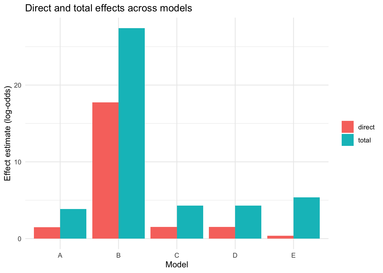
This figure helps show whether Model A remains the strongest specification in the subset, or whether one of the other published figure structures captures more of the retinal-injury signal.
We now compare our subset-based estimates with the published coefficients shown in Figures A-E. This lets us see, model by model, whether the subset reproduces the overall pattern of direct and mediated effects even if the numerical values are not identical.
boos_effect_tbl <- tibble::tribble(
  ~model, ~effect, ~boos_estimate, ~boos_se,
  "A", "indirect__diffuse_HIE", 0.834, 0.198,
  "A", "indirect__extra_axial_blood", 0.503, 0.589,
  "A", "direct", 2.431, 0.370,
  "A", "total", 3.768, NA_real_,
  "B", "indirect__extra_axial_blood", 0.464, 0.118,
  "B", "indirect__clinical_hypoxia_ischemia", 0.448, 0.168,
  "B", "indirect__diffuse_HIE", 0.386, 0.109,
  "B", "indirect__seizure", 0.272, 0.094,
  "B", "direct", 1.701, 0.308,
  "B", "total", 3.271, NA_real_,
  "C", "indirect__duration_altered_consciousness", 0.589, 0.269,
  "C", "indirect__extra_axial_blood", 0.273, 0.099,
  "C", "indirect__clinical_hypoxia_ischemia", 0.268, 0.197,
  "C", "indirect__seizure", 0.190, 0.054,
  "C", "direct", 0.936, 0.247,
  "C", "total", 2.256, NA_real_,
  "D", "indirect__duration_altered_consciousness", 0.486, 0.213,
  "D", "indirect__clinical_hypoxia_ischemia", 0.295, 0.106,
  "D", "indirect__extra_axial_blood", 0.270, 0.079,
  "D", "indirect__seizure", 0.184, 0.059,
  "D", "direct", 0.889, 0.209,
  "D", "total", 2.124, NA_real_,
  "E", "indirect__duration_altered_consciousness", 0.591, 0.201,
  "E", "indirect__diffuse_HIE", 0.437, 0.108,
  "E", "indirect__seizure", 0.200, 0.055,
  "E", "indirect__extra_axial_blood", 0.137, 0.076,
  "E", "direct", 0.604, 0.213,
  "E", "total", 1.969, NA_real_
) |>
  left_join(
    effect_tbl_long |>
      select(model, effect, subset_estimate = estimate, subset_se = se, subset_ci_lower = ci_lower, subset_ci_upper = ci_upper),
    by = c("model", "effect")
  ) |>
  mutate(
    absolute_difference = subset_estimate - boos_estimate,
    percent_of_boos = 100 * subset_estimate / boos_estimate,
    effect = sub("^indirect__", "Indirect via ", effect),
    effect = gsub("_", " ", effect),
    effect = if_else(effect == "direct", "Direct", effect),
    effect = if_else(effect == "total", "Total", effect)
  )

kable(
  boos_effect_tbl,
  digits = 3,
  caption = "Table 4. Comparison of subset-based estimates with the published Boos Figure A-E coefficients"
)| model | effect | boos_estimate | boos_se | subset_estimate | subset_se | subset_ci_lower | subset_ci_upper | absolute_difference | percent_of_boos |
|---|---|---|---|---|---|---|---|---|---|
| A | Indirect via diffuse HIE | 0.834 | 0.198 | 0.467 | 0.700 | -0.972 | 1.849 | -0.367 | 56.040 |
| A | Indirect via extra axial blood | 0.503 | 0.589 | 1.914 | 5.833 | 0.341 | 17.922 | 1.411 | 380.551 |
| A | Direct | 2.431 | 0.370 | 1.490 | 0.336 | 0.955 | 2.149 | -0.941 | 61.297 |
| A | Total | 3.768 | NA | 3.872 | 5.777 | 1.625 | 21.372 | 0.104 | 102.751 |
| B | Indirect via extra axial blood | 0.464 | 0.118 | 1.201 | 2.304 | -0.742 | 3.284 | 0.737 | 258.895 |
| B | Indirect via clinical hypoxia ischemia | 0.448 | 0.168 | 2.009 | 0.969 | 0.744 | 4.234 | 1.561 | 448.362 |
| B | Indirect via diffuse HIE | 0.386 | 0.109 | 5.046 | 9.129 | 2.532 | 34.426 | 4.660 | 1307.290 |
| B | Indirect via seizure | 0.272 | 0.094 | 1.421 | 0.732 | 0.148 | 2.874 | 1.149 | 522.272 |
| B | Direct | 1.701 | 0.308 | 17.743 | 0.334 | 17.120 | 18.297 | 16.042 | 1043.111 |
| B | Total | 3.271 | NA | 27.420 | 9.362 | 23.855 | 57.403 | 24.149 | 838.275 |
| C | Indirect via duration altered consciousness | 0.589 | 0.269 | 0.663 | 0.305 | 0.149 | 1.291 | 0.074 | 112.530 |
| C | Indirect via extra axial blood | 0.273 | 0.099 | 0.656 | 3.275 | -0.442 | 3.396 | 0.383 | 240.419 |
| C | Indirect via clinical hypoxia ischemia | 0.268 | 0.197 | 0.898 | 1.088 | -1.114 | 2.950 | 0.630 | 334.970 |
| C | Indirect via seizure | 0.190 | 0.054 | 0.578 | 0.343 | 0.095 | 1.420 | 0.388 | 303.965 |
| C | Direct | 0.936 | 0.247 | 1.520 | 0.376 | 0.858 | 2.295 | 0.584 | 162.409 |
| C | Total | 2.256 | NA | 4.315 | 3.387 | 2.393 | 7.603 | 2.059 | 191.248 |
| D | Indirect via duration altered consciousness | 0.486 | 0.213 | 0.663 | 0.320 | 0.078 | 1.300 | 0.177 | 136.379 |
| D | Indirect via clinical hypoxia ischemia | 0.295 | 0.106 | 0.898 | 1.091 | -1.309 | 2.870 | 0.603 | 304.311 |
| D | Indirect via extra axial blood | 0.270 | 0.079 | 0.656 | 1.026 | -0.578 | 3.441 | 0.386 | 243.090 |
| D | Indirect via seizure | 0.184 | 0.059 | 0.578 | 0.354 | 0.138 | 1.463 | 0.394 | 313.877 |
| D | Direct | 0.889 | 0.209 | 1.520 | 0.388 | 0.856 | 2.264 | 0.631 | 170.996 |
| D | Total | 2.124 | NA | 4.315 | 1.457 | 1.952 | 7.779 | 2.191 | 203.133 |
| E | Indirect via duration altered consciousness | 0.591 | 0.201 | 0.806 | 0.366 | 0.081 | 1.579 | 0.215 | 136.296 |
| E | Indirect via diffuse HIE | 0.437 | 0.108 | 3.586 | 1.022 | 2.068 | 6.150 | 3.149 | 820.526 |
| E | Indirect via seizure | 0.200 | 0.055 | 1.077 | 0.517 | 0.158 | 2.173 | 0.877 | 538.595 |
| E | Indirect via extra axial blood | 0.137 | 0.076 | -0.459 | 0.855 | -2.078 | 1.056 | -0.596 | -335.221 |
| E | Direct | 0.604 | 0.213 | 0.381 | 0.447 | -0.421 | 1.152 | -0.223 | 63.011 |
| E | Total | 1.969 | NA | 5.390 | 1.395 | 3.098 | 8.359 | 3.421 | 273.729 |
Table 4 is meant to show whether the subset-based replication lands in the same general range as the published figures, even though the subset is smaller and some variable definitions remain reconstructed rather than verified from the full study codebook.
We now visualize the direct and total effects from the published figures alongside the subset-based estimates so the overall agreement can be judged more quickly than from the table alone.
boos_vs_subset_plot_tbl <- boos_effect_tbl |>
  filter(effect %in% c("Direct", "Total")) |>
  transmute(
    model,
    effect,
    `Boos et al.` = boos_estimate,
    `Subset replication` = subset_estimate,
    boos_se,
    subset_ci_lower,
    subset_ci_upper
  ) |>
  pivot_longer(
    cols = c(`Boos et al.`, `Subset replication`),
    names_to = "source",
    values_to = "estimate"
  ) |>
  mutate(
    ci_lower = case_when(
      source == "Boos et al." & !is.na(boos_se) ~ estimate - 1.96 * boos_se,
      source == "Subset replication" ~ subset_ci_lower,
      TRUE ~ NA_real_
    ),
    ci_upper = case_when(
      source == "Boos et al." & !is.na(boos_se) ~ estimate + 1.96 * boos_se,
      source == "Subset replication" ~ subset_ci_upper,
      TRUE ~ NA_real_
    )
  )

ggplot(boos_vs_subset_plot_tbl, aes(x = model, y = estimate, fill = source)) +
  geom_col(position = "dodge") +
  geom_errorbar(
    aes(ymin = ci_lower, ymax = ci_upper),
    position = position_dodge(width = 0.9),
    width = 0.2,
    na.rm = TRUE
  ) +
  facet_wrap(~ effect) +
  labs(
    title = "Direct and total effects: published versus subset-based estimates",
    x = "Model",
    y = "Effect estimate (log-odds)",
    fill = NULL
  ) +
  theme_minimal()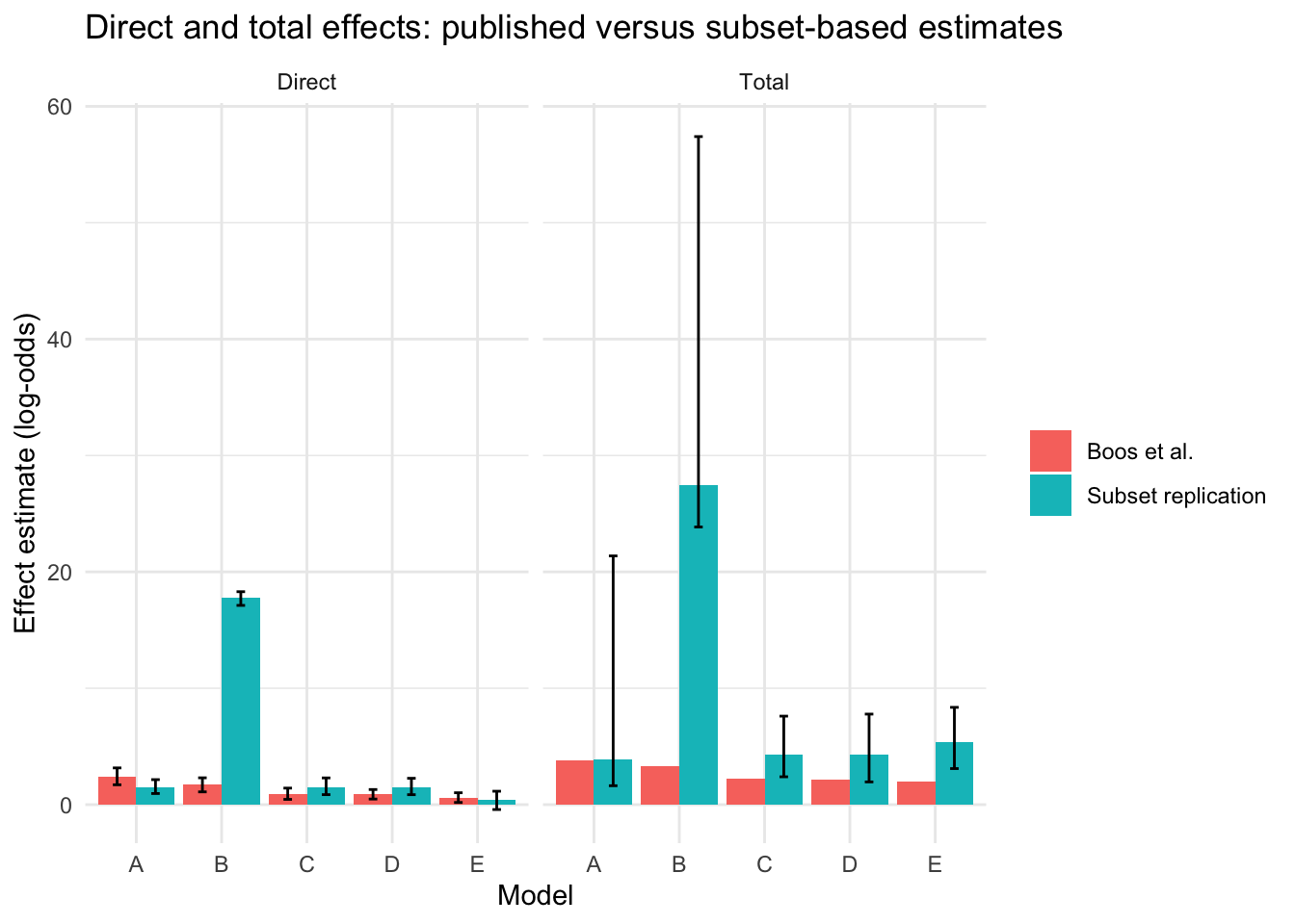
This figure helps show whether the subset-based replication preserves the broad ranking and scale of the published direct and total effects, even when the exact values differ.
Model B stands out because the subset-based replication produces a much larger direct and total effect than the published Boos figure. In this case, the most likely explanation is model instability rather than a substantively larger effect in the subset. When the Model B outcome regression was examined directly, the coefficient for inertial_injury was extremely large (17.743) and was paired with an extremely large standard error (808.473), which is a classic sign of quasi-separation or near-separation in logistic regression. In other words, the Model B regression appears to be behaving as though inertial_injury almost perfectly separates patients with and without severe retinal injury in this subset, which makes the fitted direct effect unstable and artificially large. The other Model B coefficients were far more ordinary in size and precision, so the inflation appears to be concentrated in the direct-effect term rather than spread across the whole model. For that reason, the large Model B bar in the replication should be interpreted as evidence of instability in the subset fit, not as evidence that the corresponding causal effect is truly much larger than in the published paper.
We now display the fitted Model A outcome coefficients so it is clear which variables are driving the direct and mediated paths in the closest paper-match specification.
outcome_coef_tbl <- as.data.frame(coef(summary(outcome_model))) |>
  tibble::rownames_to_column("term") |>
  rename(
    estimate = Estimate,
    std_error = `Std. Error`,
    statistic = `z value`,
    p_value = `Pr(>|z|)`
  )

kable(outcome_coef_tbl, digits = 3, caption = "Table 5. Model A outcome-model coefficients")| term | estimate | std_error | statistic | p_value |
|---|---|---|---|---|
| (Intercept) | -3.151 | 0.673 | -4.679 | 0.00 |
| isolated_inertial_injury | 1.490 | 0.298 | 4.999 | 0.00 |
| diffuse_HIE | 2.485 | 0.306 | 8.109 | 0.00 |
| extra_axial_blood | 1.509 | 0.647 | 2.331 | 0.02 |
This table is helpful because it separates the direct effect of isolated inertial injury from the associations of the two mediators with severe retinal injury.
We now plot the Model A direct and indirect effects to make the relative sizes easier to compare visually.
effect_tbl_model_a <- effect_tbl_long |>
  filter(model == "A") |>
  mutate(
    ci_lower = apply(model_results[["A"]]$boot[, effect, drop = FALSE], 2, quantile, probs = 0.025),
    ci_upper = apply(model_results[["A"]]$boot[, effect, drop = FALSE], 2, quantile, probs = 0.975)
  ) |>
  select(effect, estimate, ci_lower, ci_upper) |>
  mutate(
    effect = recode(
      effect,
      "indirect__diffuse_HIE" = "Indirect via diffuse_HIE",
      "indirect__extra_axial_blood" = "Indirect via extra_axial_blood",
      direct = "Direct",
      total = "Total"
    )
  )

ggplot(effect_tbl_model_a, aes(x = effect, y = estimate)) +
  geom_col(fill = "#3C6E71") +
  geom_errorbar(aes(ymin = ci_lower, ymax = ci_upper), width = 0.15) +
  geom_hline(yintercept = 0, linetype = "dashed", color = "grey40") +
  labs(
    title = "Direct and indirect effects",
    x = NULL,
    y = "Effect estimate (log-odds)"
  ) +
  theme_minimal()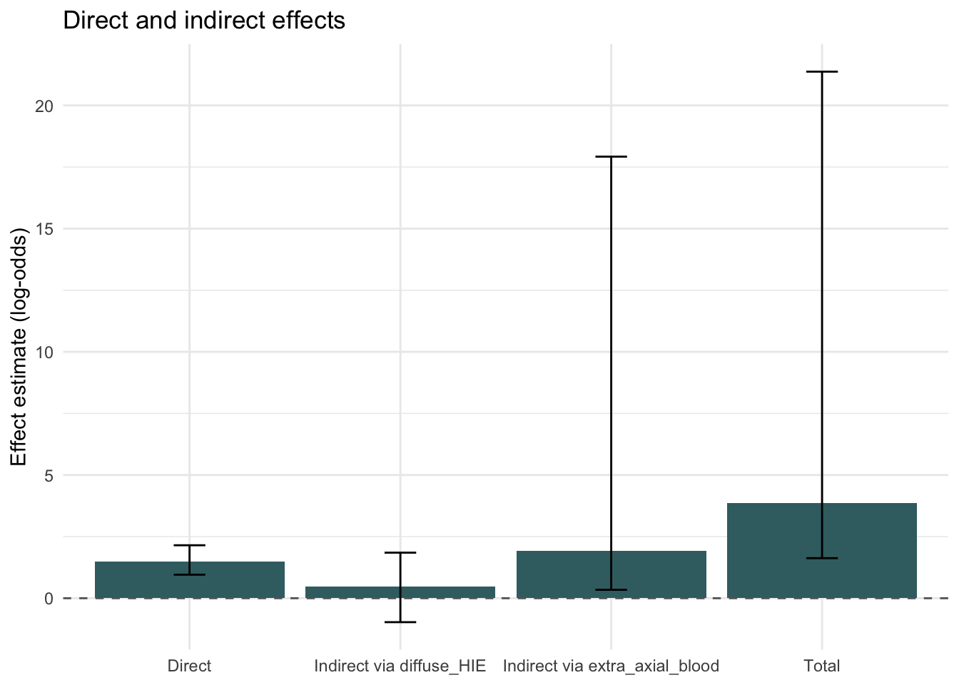
This figure helps show whether Model A is being driven mainly by the direct path from isolated inertial injury to severe retinal injury, or by the indirect paths through diffuse HIE and extra-axial blood.
We now recreate the first Boos 2025 mediation figure using the subset-based Model A estimates from this replication.

We now show parallel diagram recreations for Models B-E using the same visual style as the Model A replication figure. These panels make it easier to compare the structure and relative path magnitudes across the five published mediation models.


We next summarize the FCI search on the eight-variable union drawn from Models A-E: isolated_inertial_injury, inertial_injury, diffuse_HIE, clinical_hypoxia_ischemia, duration_altered_consciousness, extra_axial_blood, seizure, and severe_retinal_injury. Using the 312 complete cases available on that combined variable set, the estimated PAG was very sparse. The algorithm retained only two adjacencies: isolated_inertial_injury o-o inertial_injury and diffuse_HIE o-o severe_retinal_injury. No other edges were retained. This means that, in this subset, the broader FCI search did not recover a rich causal graph resembling any of the hand-specified mediation models. A practical limitation is that the discrete conditional-independence testing produced warnings that the sample size was too small for some of the higher-dimensional tests, and those cases were treated as independence, so this eight-variable PAG should be interpreted cautiously as an underpowered exploratory result rather than a definitive causal model.

We next compare the corresponding PC and GES searches on the same eight-variable union. The PC algorithm returned a small non-empty graph, retaining the edges isolated_inertial_injury --> inertial_injury, inertial_injury --> severe_retinal_injury, duration_altered_consciousness --> inertial_injury, diffuse_HIE --> severe_retinal_injury, and two unoriented adjacencies involving duration_altered_consciousness, namely diffuse_HIE --- duration_altered_consciousness and clinical_hypoxia_ischemia --- duration_altered_consciousness. By contrast, the GES run returned an empty graph under the available Gaussian score approximation. Taken together, these results suggest that the eight-variable causal search is highly sensitive to algorithm choice in this subset, with FCI returning a very sparse PAG, PC retaining a small directed graph, and GES finding no edges at all.

This replication should be read as an informed approximation, not as a definitive reproduction of the published Boos 2025 mediation model. The main reasons are that the full paper dataset was not available, the exact mediation-figure specification could only be inferred from the paper abstract and snippets, and some variable definitions, especially the HIE depth and distribution mapping, remain partly reconstructed rather than verified from a codebook.
Within those limits, this file provides a transparent first-pass implementation of the model that appears to be summarized in the abstract: isolated inertial injury as the primary exposure, diffuse HIE and extra-axial blood as mediators, and severe retinal injury as the outcome among children with ophthalmology examinations.
Models A-E are best understood as alternative causal specifications built from largely the same set of clinical variables, rather than as five entirely different analyses. Across the five models, the outcome remains severe retinal injury, but variables such as isolated inertial injury, inertial injury, diffuse HIE, clinical hypoxia or ischemia, duration of altered consciousness, extra-axial blood, and seizure are reassigned to different roles as primary exposures or mediators. In that sense, the models are permutations of a shared variable set, but they are not merely arbitrary reorderings. Each model encodes a different hypothesized causal mechanism for how severe retinal injury might arise, and the purpose of comparing them is to see which arrangement of the same core variables provides the most explanatory account of the observed data.