Two-Part Statistical Analysis of NIFM Occurrence and Mark Informativeness
Author
Maria Cuellar
Published
March 17, 2026
1 Purpose
This report starts the substantive statistical analysis for the Stoney NIJ project using the most recent grouped data currently present in this project directory. The main modeling idea is a two-part or hurdle-style analysis.
That framing is natural here because the scientifically relevant outcome has two stages:
many tested rounds yield no observed NIFM at all
among rounds with a NIFM, the mark can then vary in informativeness
A single model for raw minutiae counts would mix those two processes together. For this project, it is more interpretable to separate:
NIFM occurrence: does a round yield any NIFM?
mark informativeness: conditional on a NIFM being present, how strong is that mark?
This report uses grouped counts, so the results should be treated as category-level analyses. They are useful for identifying broad patterns, but they do not yet account for clustering within guns, donors, or loads. With round-level data, the same two-part logic could be implemented more formally as an individual-level hurdle model.
2 Data
The current analysis uses data/nifm-2-12-25.csv. Each row is a handgun type / caliber category. The Rounds Tested column gives the total number of rounds in that category. The remaining count columns give the number of observed NIFMs with each minutiae count.
Now load the grouped data and create the derived variables used throughout the rest of the analysis.
Grouped summary statistics by handgun type and caliber.
group
Type
Caliber
Rounds Tested
Donors
total_nifm
occurrence_rate
mean_minutiae
p_ge_6
p_ge_8
p_ge_10
A22
A
22
198
15
50
0.253
5.30
0.400
0.060
0.020
A32
A
32
105
12
60
0.571
5.63
0.417
0.133
0.067
A38
A
38
348
20
101
0.290
5.44
0.347
0.119
0.020
A45
A
45
178
16
50
0.281
5.16
0.260
0.100
0.000
R22
R
22
225
23
52
0.231
5.29
0.327
0.115
0.038
R38
R
38
107
20
79
0.738
5.85
0.342
0.203
0.114
R45
R
45
102
12
86
0.843
5.79
0.337
0.221
0.081
3 Why A Two-Part Model Makes Sense
At the round level, the outcome of interest is effectively zero-inflated in the ordinary-language sense: many rounds have zero observed NIFMs, while positive rounds have a right-skewed positive outcome.
For this dataset, a hurdle interpretation is more natural than a classic zero-inflated Poisson interpretation:
the zero state is scientifically meaningful, not just a technical nuisance
the positive state has its own scientific meaning because the quality of the observed NIFM matters
So the main analysis below is organized in two parts:
Part 1 models whether any NIFM occurs
Part 2 models whether the observed NIFM is more informative, using minutiae >= 8 as the primary threshold
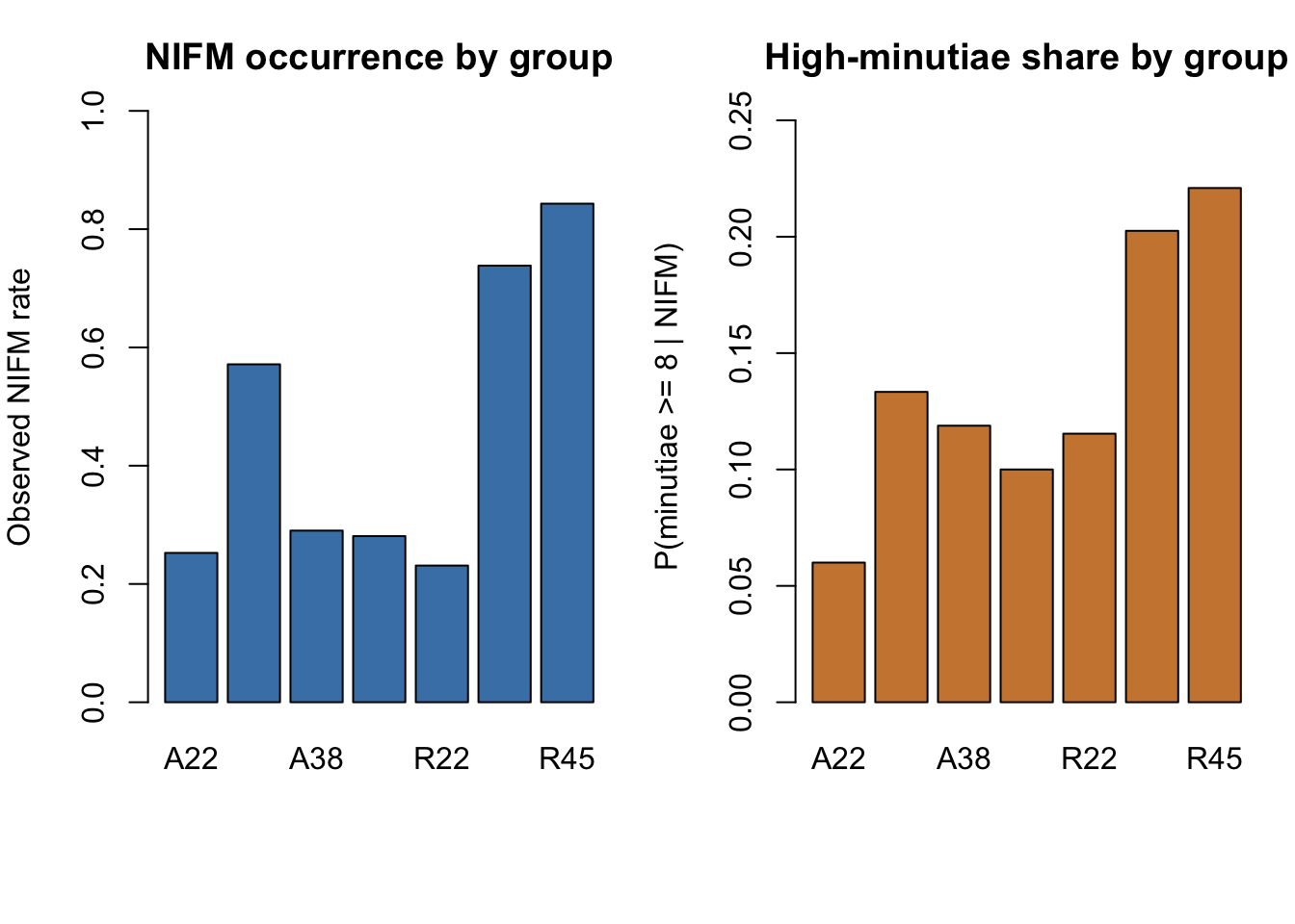
4 Descriptive Patterns
The table above already shows two notable patterns.
The rate of NIFM occurrence varies widely by category, from about 23% in R22 to about 84% in R45.
The average minutiae count among observed NIFMs is more stable, ranging from about 5.16 to 5.85, but the share of higher-minutiae NIFMs appears larger in the revolver categories R38 and R45.
Now plot those two patterns directly so the separation between occurrence and informativeness is easy to see.
For the first part of the hurdle model, the natural data structure is grouped binomial: each row gives the number of NIFMs observed out of the total number of tested rounds in that category.
5.1 Global Heterogeneity Test
Now test whether the seven groups have the same overall NIFM occurrence rate.
Code
occurrence_table <-as.matrix(dat[, c("total_nifm", "no_nifm")])rownames(occurrence_table) <- dat$groupcolnames(occurrence_table) <-c("NIFM", "No NIFM")occurrence_chisq <-chisq.test(occurrence_table)occurrence_chisq
This test strongly rejects equal occurrence rates across the seven groups.
5.2 Group-Specific Occurrence Estimates
The simplest category-level version of Part 1 is a grouped-binomial model with one parameter per handgun-type / caliber group. This is just a convenient way to estimate the observed occurrence rates on the log-odds scale.
Now estimate the group-specific occurrence levels on the log-odds scale.
Code
occurrence_fit_group <-glm(cbind(total_nifm, no_nifm) ~0+ group,data = dat,family =binomial())occurrence_coef <-data.frame(group = dat$group,occurrence_rate =round(dat$occurrence_rate, 3),log_odds =round(coef(occurrence_fit_group), 3))knitr::kable( occurrence_coef,caption ="Group-specific occurrence estimates for Part 1 of the two-part analysis.")
Group-specific occurrence estimates for Part 1 of the two-part analysis.
group
occurrence_rate
log_odds
groupA22
A22
0.253
-1.085
groupA32
A32
0.571
0.288
groupA38
A38
0.290
-0.894
groupA45
A45
0.281
-0.940
groupR22
R22
0.231
-1.202
groupR38
R38
0.738
1.037
groupR45
R45
0.843
1.682
5.3 Exploratory Main-Effects Grouped-Binomial Model
Because there are only seven grouped rows, any regression decomposition is exploratory. As a first pass, I fit a main-effects model with handgun type and caliber:
Now fit a simpler explanatory model that separates handgun type from caliber.
Code
occurrence_fit <-glm(cbind(total_nifm, no_nifm) ~ Type +factor(Caliber),data = dat,family =quasibinomial())summary(occurrence_fit)
Call:
glm(formula = cbind(total_nifm, no_nifm) ~ Type + factor(Caliber),
    family = quasibinomial(), data = dat)

Coefficients:
                  Estimate Std. Error t value Pr(>|t|)
(Intercept)        -1.9756     0.9059  -2.181    0.161
TypeR               1.3396     0.8404   1.594    0.252
factor(Caliber)32   2.2633     1.4607   1.549    0.261
factor(Caliber)38   1.2208     0.9773   1.249    0.338
factor(Caliber)45   1.4371     1.0462   1.374    0.303

(Dispersion parameter for quasibinomial family taken to be 33.76481)

    Null deviance: 222.783  on 6  degrees of freedom
Residual deviance:  63.977  on 2  degrees of freedom
AIC: NA

Number of Fisher Scoring iterations: 4
Code
occurrence_fitted <-data.frame(group = dat$group,observed =round(dat$occurrence_rate, 3),fitted =round(fitted(occurrence_fit), 3))knitr::kable( occurrence_fitted,caption ="Observed and fitted NIFM occurrence rates from the exploratory grouped-binomial model.")
Observed and fitted NIFM occurrence rates from the exploratory grouped-binomial model.
group
observed
fitted
A22
0.253
0.122
A32
0.571
0.571
A38
0.290
0.320
A45
0.281
0.369
R22
0.231
0.346
R38
0.738
0.642
R45
0.843
0.690
The main conclusion from this model is not that any single coefficient is precisely estimated; with only seven grouped rows, coefficient-level inference is fragile. The useful takeaway is that the data clearly show between-group heterogeneity in Part 1 of the hurdle model.
6 Part 2: Mark Informativeness Among Observed NIFMs
For the second part of the hurdle model, the question is no longer whether a NIFM exists. Instead, conditional on observing a NIFM, the question is whether some groups tend to produce more informative marks.
The raw minutiae categories are sparse in the upper tail, so I use coarser bands:
4_5
6_7
8plus
6.1 Three-Band Distribution Test
Now compare the full low-versus-mid-versus-high minutiae distribution across groups.
Code
band_table <-cbind(`4_5`=rowSums(count_matrix[, minutiae_values %in%c(4, 5), drop =FALSE]),`6_7`=rowSums(count_matrix[, minutiae_values %in%c(6, 7), drop =FALSE]),`8plus`=rowSums(count_matrix[, minutiae_values >=8, drop =FALSE]))rownames(band_table) <- dat$groupband_chisq <-chisq.test(band_table, simulate.p.value =TRUE, B =100000)band_chisq
    Pearson's Chi-squared test with simulated p-value (based on 1e+05
    replicates)

data:  band_table
X-squared = 22.671, df = NA, p-value = 0.02899
Code
knitr::kable(cbind(group =rownames(band_table), as.data.frame(band_table)),caption ="Observed minutiae-count bands among NIFMs by group.")
Observed minutiae-count bands among NIFMs by group.
group
4_5
6_7
8plus
A22
A22
30
17
3
A32
A32
35
17
8
A38
A38
66
23
12
A45
A45
37
8
5
R22
R22
35
11
6
R38
R38
52
11
16
R45
R45
57
10
19
This provides evidence that the minutiae distribution differs across groups, although the effect is more modest than the group differences in overall NIFM occurrence.
6.2 Focused High-Minutiae Analysis
Because David’s notes emphasize the practical value of more informative marks, I also examine the probability that an observed NIFM has at least 8 minutiae.
Now focus on the more practical threshold question: among observed NIFMs, how often does a mark reach at least 8 minutiae?
Call:
glm(formula = cbind(nifm_ge_8, total_nifm - nifm_ge_8) ~ Type +
    factor(Caliber), family = quasibinomial(), data = dat)

Coefficients:
                  Estimate Std. Error t value Pr(>|t|)
(Intercept)       -2.77098    0.12760 -21.717  0.00211 **
TypeR              0.74429    0.09455   7.872  0.01576 *
factor(Caliber)32  0.89917    0.17553   5.123  0.03606 *
factor(Caliber)38  0.70544    0.12968   5.440  0.03217 *
factor(Caliber)45  0.71900    0.13282   5.414  0.03247 *
---
Signif. codes:  0 '***' 0.001 '**' 0.01 '*' 0.05 '.' 0.1 ' ' 1

(Dispersion parameter for quasibinomial family taken to be 0.1007278)

    Null deviance: 11.01845  on 6  degrees of freedom
Residual deviance:  0.20439  on 2  degrees of freedom
AIC: NA

Number of Fisher Scoring iterations: 3
Code
high_fitted <-data.frame(group = dat$group,total_nifm = dat$total_nifm,observed =round(dat$p_ge_8, 3),fitted =round(fitted(high_fit), 3))knitr::kable( high_fitted,caption ="Observed and fitted probabilities that an observed NIFM has at least 8 minutiae.")
Observed and fitted probabilities that an observed NIFM has at least 8 minutiae.
group
total_nifm
observed
fitted
A22
50
0.060
0.059
A32
60
0.133
0.133
A38
101
0.119
0.112
A45
50
0.100
0.114
R22
52
0.115
0.116
R38
79
0.203
0.211
R45
86
0.221
0.213
The simple chi-square test is suggestive but not definitive at the 0.05 level, while the exploratory main-effects model points in the same direction: revolver categories appear to yield a larger share of high-minutiae NIFMs than automatic categories, especially in R38 and R45.
7 Two-Part Interpretation
Taken together, the two-part results suggest that category differences operate more strongly through NIFM occurrence than through minutiae quality alone.
More specifically:
Part 1 is the strongest signal in the data: some categories are much more likely than others to produce any NIFM.
Part 2 also shows group differences, but they are more modest: among observed NIFMs, some groups appear more likely to produce marks with at least 8 minutiae.
This means a category can be scientifically favorable for two different reasons:
it yields NIFMs often
or, when it yields them, they tend to be more informative
That distinction is exactly why the two-part framework is better suited to this problem than a single omnibus count model.
8 Interpretation
At this stage, the strongest empirical result is:
The categories differ substantially in how often NIFMs occur at all.
A secondary result is:
The categories may also differ in the quality distribution of observed NIFMs, with some revolver categories producing a larger fraction of higher-minutiae marks.
By contrast:
The average minutiae count alone does not appear to separate the groups as strongly as the two-part analysis does.
9 Limitations
These analyses are a good starting point, but there are important limits to what can be claimed from the current file alone.
The data are aggregated by category, so there is no adjustment for within-gun, within-donor, or within-load dependence.
The absent R32 category is a structural gap and is not modeled directly here.
The grouped main-effects models are exploratory because there are only seven category-level rows.
The current data do not yet incorporate ESLR or any direct measure of associative value.
Because the data are aggregated, this is a grouped approximation to a hurdle model, not the full individual-round version.
10 Recommended Next Analysis Steps
The next most useful extensions are:
Create a round-level dataset if those underlying records exist.
Fit the same two-part model at the round level, with random effects for donor and gun if available.
Model higher-detail marks directly, for example minutiae >= 8 or minutiae >= 10.
Incorporate ESLR or another selectivity measure once those values are available.
Decide whether the scientific target is best framed as:
occurrence of any NIFM,
occurrence of a sufficiently informative NIFM,
or total evidential yield per load.
For now, this report gives a reproducible baseline analysis that is much closer to the actual project questions than the earlier power-only draft, and it does so in the two-part framework that best matches the zero-heavy structure of the outcome.